Calculating Federal and State Income Taxes
Shane Orr
Source:vignettes/using-usincometaxes.Rmd
using-usincometaxes.RmdThis article presents two use cases for usincometaxes.
The first shows users how to estimate income taxes from a data frame
containing financial information and other characteristics of tax payer
units. This income could come from surveys such as the Consumer Expenditure survey or the
Panel Study of Income
Dynamics survey. The second use case focuses on running
simulations.
Calculating income taxes from survey data
For the first example we will use an internal data set called
taxpayer_finances. The data is randomly generated and
formatted for use with usincometaxes. Guidance on
formatting data can be found in the Description of Input Columns article.
The data set contains financial and other household characteristics that help estimate income taxes.
| taxsimid | year | mstat | state | page | sage | depx | age1 | age2 | age3 | pwages | swages | dividends | intrec | stcg | ltcg |
|---|---|---|---|---|---|---|---|---|---|---|---|---|---|---|---|
| 1 | 2000 | single | NC | 37 | 0 | 4 | 6 | 7 | 8 | 26361.75 | 0.00 | 2260.86 | 4340.19 | 2280.16 | 2060.29 |
| 2 | 2000 | single | NC | 29 | 0 | 1 | 7 | 0 | 0 | 33966.34 | 0.00 | 1969.54 | 868.10 | 1064.50 | 2234.61 |
| 3 | 2000 | married, jointly | NC | 36 | 30 | 1 | 13 | 0 | 0 | 174191.53 | 102286.98 | 1972.47 | 2048.31 | 1009.11 | 1226.34 |
| 4 | 2000 | married, jointly | NC | 37 | 34 | 3 | 5 | 6 | 7 | 67604.57 | 53205.76 | 1173.95 | 881.67 | 3582.74 | 1405.74 |
| 5 | 2000 | married, jointly | NC | 38 | 39 | 0 | 0 | 0 | 0 | 21176.78 | 21687.72 | 4614.91 | 1588.52 | 560.93 | 825.04 |
| 6 | 2000 | single | NC | 36 | 0 | 1 | 2 | 0 | 0 | 53397.72 | 0.00 | 2067.41 | 1320.01 | 687.23 | 3548.07 |
Each row in the data set is a tax paying unit. Thus, each row files one tax return. Columns represent items reported on tax returns that impact taxes. Of course, the information in the data set does not represent everything people report on tax returns. For this reason, the income tax calculations are simply estimates.
We call taxsim_calculate_taxes() to estimate federal and
state income taxes for each tax paying unit. We are only interested in
federal and state tax liabilities, not line item credits and deduction,
so we are using return_all_information = FALSE.
family_taxes <- taxsim_calculate_taxes(
  .data = taxpayer_finances,
  return_all_information = FALSE
)

family_taxes %>%
  head() %>%
kable()| taxsimid | fiitax | siitax | fica | frate | srate | ficar | tfica |
|---|---|---|---|---|---|---|---|
| 1 | 924.97 | 1078.23 | 4033.35 | 15.00 | 7.00 | 15.3 | 2016.67 |
| 2 | 3596.23 | 1919.22 | 5196.85 | 15.00 | 7.00 | 15.3 | 2598.42 |
| 3 | 78080.32 | 20429.27 | 26915.48 | 36.58 | 8.12 | 2.9 | 13457.74 |
| 4 | 23279.56 | 7783.72 | 18483.98 | 30.83 | 7.75 | 15.3 | 9241.99 |
| 5 | 5584.33 | 2619.27 | 6558.27 | 15.00 | 7.00 | 15.3 | 3279.13 |
| 6 | 8358.38 | 3383.43 | 8169.85 | 28.00 | 7.00 | 15.3 | 4084.93 |
The taxsimid column is required for any input data frame
used in taxsim_calculate_taxes. This column is also
returned in the output data frame containing tax calculations, allowing
us to link the input and output data frames.
income_and_taxes <- taxpayer_finances %>%
  left_join(family_taxes, by = 'taxsimid')

income_and_taxes %>%
  head() %>%
kable()| taxsimid | year | mstat | state | page | sage | depx | age1 | age2 | age3 | pwages | swages | dividends | intrec | stcg | ltcg | fiitax | siitax | fica | frate | srate | ficar | tfica |
|---|---|---|---|---|---|---|---|---|---|---|---|---|---|---|---|---|---|---|---|---|---|---|
| 1 | 2000 | single | NC | 37 | 0 | 4 | 6 | 7 | 8 | 26361.75 | 0.00 | 2260.86 | 4340.19 | 2280.16 | 2060.29 | 924.97 | 1078.23 | 4033.35 | 15.00 | 7.00 | 15.3 | 2016.67 |
| 2 | 2000 | single | NC | 29 | 0 | 1 | 7 | 0 | 0 | 33966.34 | 0.00 | 1969.54 | 868.10 | 1064.50 | 2234.61 | 3596.23 | 1919.22 | 5196.85 | 15.00 | 7.00 | 15.3 | 2598.42 |
| 3 | 2000 | married, jointly | NC | 36 | 30 | 1 | 13 | 0 | 0 | 174191.53 | 102286.98 | 1972.47 | 2048.31 | 1009.11 | 1226.34 | 78080.32 | 20429.27 | 26915.48 | 36.58 | 8.12 | 2.9 | 13457.74 |
| 4 | 2000 | married, jointly | NC | 37 | 34 | 3 | 5 | 6 | 7 | 67604.57 | 53205.76 | 1173.95 | 881.67 | 3582.74 | 1405.74 | 23279.56 | 7783.72 | 18483.98 | 30.83 | 7.75 | 15.3 | 9241.99 |
| 5 | 2000 | married, jointly | NC | 38 | 39 | 0 | 0 | 0 | 0 | 21176.78 | 21687.72 | 4614.91 | 1588.52 | 560.93 | 825.04 | 5584.33 | 2619.27 | 6558.27 | 15.00 | 7.00 | 15.3 | 3279.13 |
| 6 | 2000 | single | NC | 36 | 0 | 1 | 2 | 0 | 0 | 53397.72 | 0.00 | 2067.41 | 1320.01 | 687.23 | 3548.07 | 8358.38 | 3383.43 | 8169.85 | 28.00 | 7.00 | 15.3 | 4084.93 |
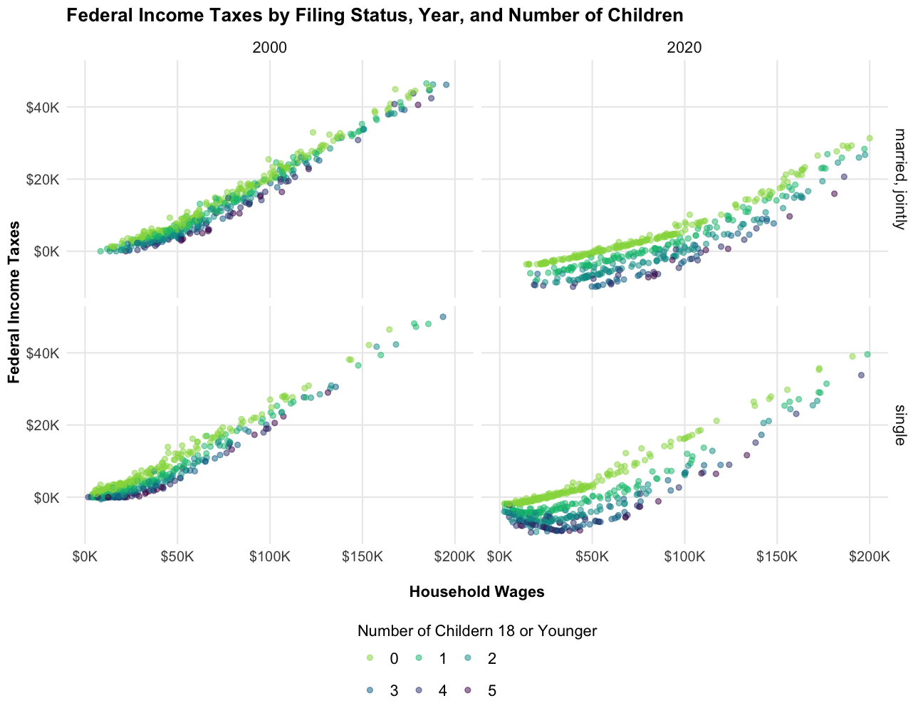
Now we have a single data frame containing both wages and income tax liabilities. Let’s take a look at the relationship between wages and estimated federal income taxes. The colors represent the number of children 18 or younger.
# custom theme for all plots in the vignette
plt_theme <- function() {

    theme_minimal() +
    theme(
      legend.text = element_text(size = 11),
      axis.text = element_text(size = 10),
      axis.title=element_text(size=11,face="bold"),
      strip.text = element_text(size = 11),
      panel.grid.minor = element_blank(),
      plot.title = element_text(face = "bold"),
      plot.subtitle = element_text(size = 12),
      legend.position = 'bottom'
    )
}
# color palettes for number of children
dep_color_palette <- rev(c('#4B0055','#353E7C','#007094','#009B95','#00BE7D','#96D84B'))

income_and_taxes %>%
  mutate(
    tax_unit_income = pwages + swages,
    num_dependents_eitc = factor(depx, levels = as.character(0:5)),
    filing_status = tools::toTitleCase(mstat)
  ) %>%
  ggplot(aes(tax_unit_income, fiitax, color = num_dependents_eitc)) +
    geom_point(alpha = .5) +
    scale_x_continuous(labels = scales::label_dollar(scale = .001, suffix = "K"), limits = c(0, 200000)) +
    scale_y_continuous(labels = scales::label_dollar(scale = .001, suffix = "K"), limits = c(-10000, 50000)) +
    scale_color_discrete(type = dep_color_palette) +
    facet_grid(rows = vars(mstat), cols = vars(year)) +
    labs(
      title = "Federal Income Taxes by Filing Status, Year, and Number of Children",
      x = "\nHousehold Wages",
      y = "Federal Income Taxes"
    ) +
    plt_theme() +
    guides(color = guide_legend(title = "Number of Childern 18 or Younger", title.position = "top", byrow = TRUE))
#> Warning: Removed 134 rows containing missing values (`geom_point()`).
The plots shows what we would expect: higher income families pay more in taxes and households pay less the more children they have. We also see the reduction in federal marginal tax rates from 2000 to 2020, as shown by the decrease in income tax liabilities when comparing the two years.
Income tax simulations
Association between income taxes paid and household wages
An additional use of usincometaxes is to run
simulations. This could be as simple as plotting the relationship
between wages and income taxes paid. To do this, we first need to create
a data set that holds everything constant except for wages. The code
block below does this, except it also creates different data sets for
households with zero and four children 18 or younger, so we can compare
differences on this characteristic as well.
# calculate taxes from 0 to 200,000 in wages
wage_linespace <- seq(0, 200000, 100)

n_kids <- 4

base_family_income <- data.frame(
  year = 2020,
  mstat = 'married, jointly',
  state = 'NC',
  page = 40,
  sage = 40,
  depx = n_kids,
  age1 = n_kids,
  age2 = n_kids,
  age3 = n_kids,
  pwages = wage_linespace,
  swages = 0
)

# create an additional data set with no dependents and add it to the original
family_income <- base_family_income %>%
  bind_rows(
    # make all numeber of dependent columns 0
    base_family_income %>%
      mutate(across(c(depx, age1, age2, age3), ~0))
  ) %>%
  # add unique ID to each row
  mutate(taxsimid = row_number()) %>%
  select(taxsimid, everything())

family_income %>%
  head() %>%
kable()| taxsimid | year | mstat | state | page | sage | depx | age1 | age2 | age3 | pwages | swages |
|---|---|---|---|---|---|---|---|---|---|---|---|
| 1 | 2020 | married, jointly | NC | 40 | 40 | 4 | 4 | 4 | 4 | 0 | 0 |
| 2 | 2020 | married, jointly | NC | 40 | 40 | 4 | 4 | 4 | 4 | 100 | 0 |
| 3 | 2020 | married, jointly | NC | 40 | 40 | 4 | 4 | 4 | 4 | 200 | 0 |
| 4 | 2020 | married, jointly | NC | 40 | 40 | 4 | 4 | 4 | 4 | 300 | 0 |
| 5 | 2020 | married, jointly | NC | 40 | 40 | 4 | 4 | 4 | 4 | 400 | 0 |
| 6 | 2020 | married, jointly | NC | 40 | 40 | 4 | 4 | 4 | 4 | 500 | 0 |
Now, we will calculate federal and state income taxes for our
simulated data set. Note that
return_all_information = TRUE. This allows us to examine
credit amounts like the Child Tax Credit and Earned Income Tax Credit
(EITC).
family_income_taxes <- taxsim_calculate_taxes(
  .data = family_income,
  return_all_information = TRUE
)

family_income_taxes %>%
  head() %>%
kable()| taxsimid | fiitax | siitax | fica | frate | srate | ficar | tfica | credits | v10_federal_agi | v11_ui_agi | v12_soc_sec_agi | v13_zero_bracket_amount | v14_personal_exemptions | v15_exemption_phaseout | v16_deduction_phaseout | v17_itemized_deductions | v18_federal_taxable_income | v19_tax_on_taxable_income | v20_exemption_surtax | v21_general_tax_credit | v22_child_tax_credit_adjusted | v23_child_tax_credit_refundable | v24_child_care_credit | v25_eitc | v26_amt_income | v27_amt_liability | v28_fed_income_tax_before_credit | v29_fica | v30_state_household_income | v31_state_rent_expense | v32_state_agi | v33_state_exemption_amount | v34_state_std_deduction_amount | v35_state_itemized_deduction | v36_state_taxable_income | v37_state_property_tax_credit | v38_state_child_care_credit | v39_state_eitc | v40_state_total_credits | v41_state_bracket_rate | staxbc | v42_self_emp_income | v43_medicare_tax_unearned_income | v44_medicare_tax_earned_income | v45_cares_recovery_rebate |
|---|---|---|---|---|---|---|---|---|---|---|---|---|---|---|---|---|---|---|---|---|---|---|---|---|---|---|---|---|---|---|---|---|---|---|---|---|---|---|---|---|---|---|---|---|---|
| 1 | -6900 | 0 | 0.0 | -45 | 0 | 15.3 | 0.00 | 0 | 0 | 0 | 0 | 24800 | 0 | 0 | 0 | 0 | 0 | 0 | 0 | 0 | 0 | 0 | 0 | 0 | 0 | 0 | 0 | 0.0 | 0.01 | 0 | 0.01 | 0 | 21500 | 0 | 0 | 0 | 0 | 0 | 0 | 0 | 0 | 0 | 0 | 0 | 6900 |
| 2 | -6945 | 0 | 15.3 | -45 | 0 | 15.3 | 7.65 | 0 | 100 | 0 | 0 | 24800 | 0 | 0 | 0 | 0 | 0 | 0 | 0 | 0 | 0 | 0 | 0 | 45 | 100 | 0 | 0 | 15.3 | 101.01 | 0 | 100.01 | 0 | 21500 | 0 | 0 | 0 | 0 | 0 | 0 | 0 | 0 | 0 | 0 | 0 | 6900 |
| 3 | -6990 | 0 | 30.6 | -45 | 0 | 15.3 | 15.30 | 0 | 200 | 0 | 0 | 24800 | 0 | 0 | 0 | 0 | 0 | 0 | 0 | 0 | 0 | 0 | 0 | 90 | 200 | 0 | 0 | 30.6 | 201.01 | 0 | 200.01 | 0 | 21500 | 0 | 0 | 0 | 0 | 0 | 0 | 0 | 0 | 0 | 0 | 0 | 6900 |
| 4 | -7035 | 0 | 45.9 | -45 | 0 | 15.3 | 22.95 | 0 | 300 | 0 | 0 | 24800 | 0 | 0 | 0 | 0 | 0 | 0 | 0 | 0 | 0 | 0 | 0 | 135 | 300 | 0 | 0 | 45.9 | 301.01 | 0 | 300.01 | 0 | 21500 | 0 | 0 | 0 | 0 | 0 | 0 | 0 | 0 | 0 | 0 | 0 | 6900 |
| 5 | -7080 | 0 | 61.2 | -45 | 0 | 15.3 | 30.60 | 0 | 400 | 0 | 0 | 24800 | 0 | 0 | 0 | 0 | 0 | 0 | 0 | 0 | 0 | 0 | 0 | 180 | 400 | 0 | 0 | 61.2 | 401.01 | 0 | 400.01 | 0 | 21500 | 0 | 0 | 0 | 0 | 0 | 0 | 0 | 0 | 0 | 0 | 0 | 6900 |
| 6 | -7125 | 0 | 76.5 | -45 | 0 | 15.3 | 38.25 | 0 | 500 | 0 | 0 | 24800 | 0 | 0 | 0 | 0 | 0 | 0 | 0 | 0 | 0 | 0 | 0 | 225 | 500 | 0 | 0 | 76.5 | 501.01 | 0 | 500.01 | 0 | 21500 | 0 | 0 | 0 | 0 | 0 | 0 | 0 | 0 | 0 | 0 | 0 | 6900 |
As before, let’s merge our tax data with the original input data set.
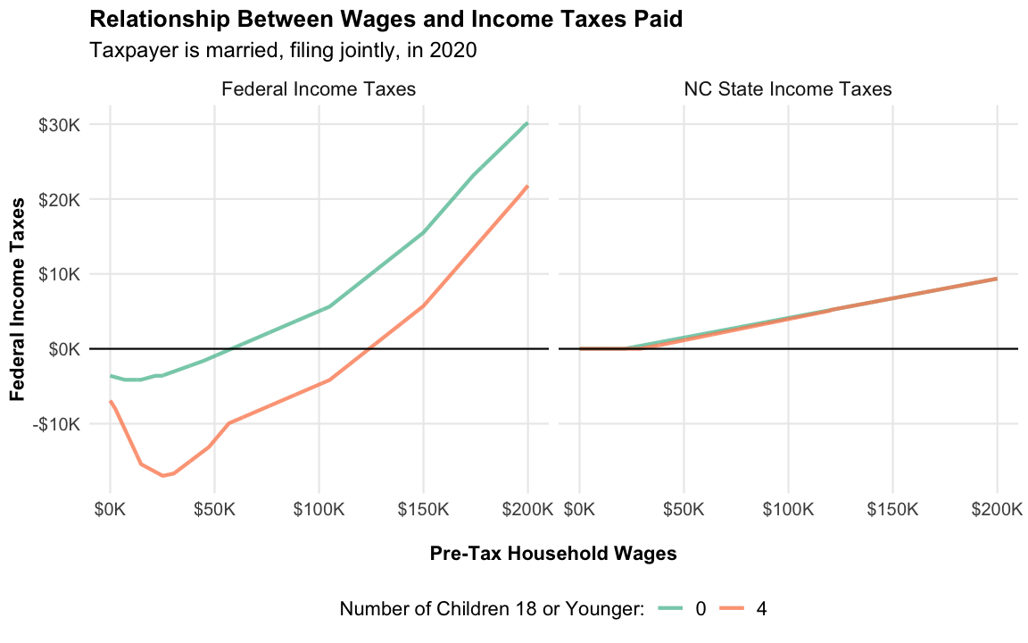
Now, let’s look at the relationship between household wages and estimated income tax liabilities.
family_income_long <- family_income %>%
  select(pwages, depx, fiitax, siitax) %>%
  pivot_longer(cols = c('fiitax', 'siitax'),
               names_to = 'jurisdiction', values_to = 'taxes_paid') %>%
  mutate(
    jurisdiction = recode(jurisdiction, 'fiitax' = 'Federal Income Taxes', 'siitax' = 'NC State Income Taxes'),
    num_dependents_eitc = factor(depx, levels = as.character(0:5)),
    post_tax_wages = pwages - taxes_paid
  )
# primary_wages, taxes_paid, color = as.character(num_dependents_eitc)
taxes_line_plot <- function(.data, x_var, y_var, color_var) {
  ggplot(.data, aes({{x_var}}, {{y_var}}, color = {{color_var}})) +
    geom_line(size = 1, alpha = .8) +
    geom_hline(yintercept = 0) +
    scale_x_continuous(labels = scales::label_dollar(scale = .001, suffix = "K")) +
    scale_y_continuous(labels = scales::label_dollar(scale = .001, suffix = "K")) +
    scale_color_brewer(type = 'seq', palette = 'Set2')  +
    plt_theme()

}
taxes_line_plot(family_income_long, pwages, taxes_paid, num_dependents_eitc) +
  facet_wrap(vars(jurisdiction)) +
  labs(
    title = "Relationship Between Wages and Income Taxes Paid",
    subtitle = "Taxpayer is married, filing jointly, in 2020",
    x = "\nPre-Tax Household Wages",
    y = "Federal Income Taxes",
    color = 'Number of Children 18 or Younger:'
  )
#> Warning: Using `size` aesthetic for lines was deprecated in ggplot2 3.4.0.
#> ℹ Please use `linewidth` instead.
#> This warning is displayed once every 8 hours.
#> Call `lifecycle::last_lifecycle_warnings()` to see where this warning was
#> generated.
Note that North Carolina had a flat tax of 5.25% in 2020. That’s why their taxes increase linearly.
Relationship Between Pre and Post-Tax Wages
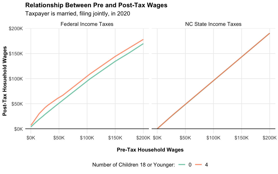
We’ll create a additional plot comparing pre-tax and post-tax household wages.
taxes_line_plot(family_income_long, pwages, post_tax_wages, num_dependents_eitc) +
  facet_wrap(vars(jurisdiction)) +
  labs(
    title = "Relationship Between Pre and Post-Tax Wages",
    subtitle = "Taxpayer is married, filing jointly, in 2020",
    x = "\nPre-Tax Household Wages",
    y = "Post-Tax Hosuehold Wages",
    color = 'Number of Children 18 or Younger:'
  )
Child Tax Credit and Earned Income Tax Credit (EITC)
As noted previously, setting
return_all_information = TRUE lets us retrieve additional
output. Included in this additional output are amounts for the Child Tax
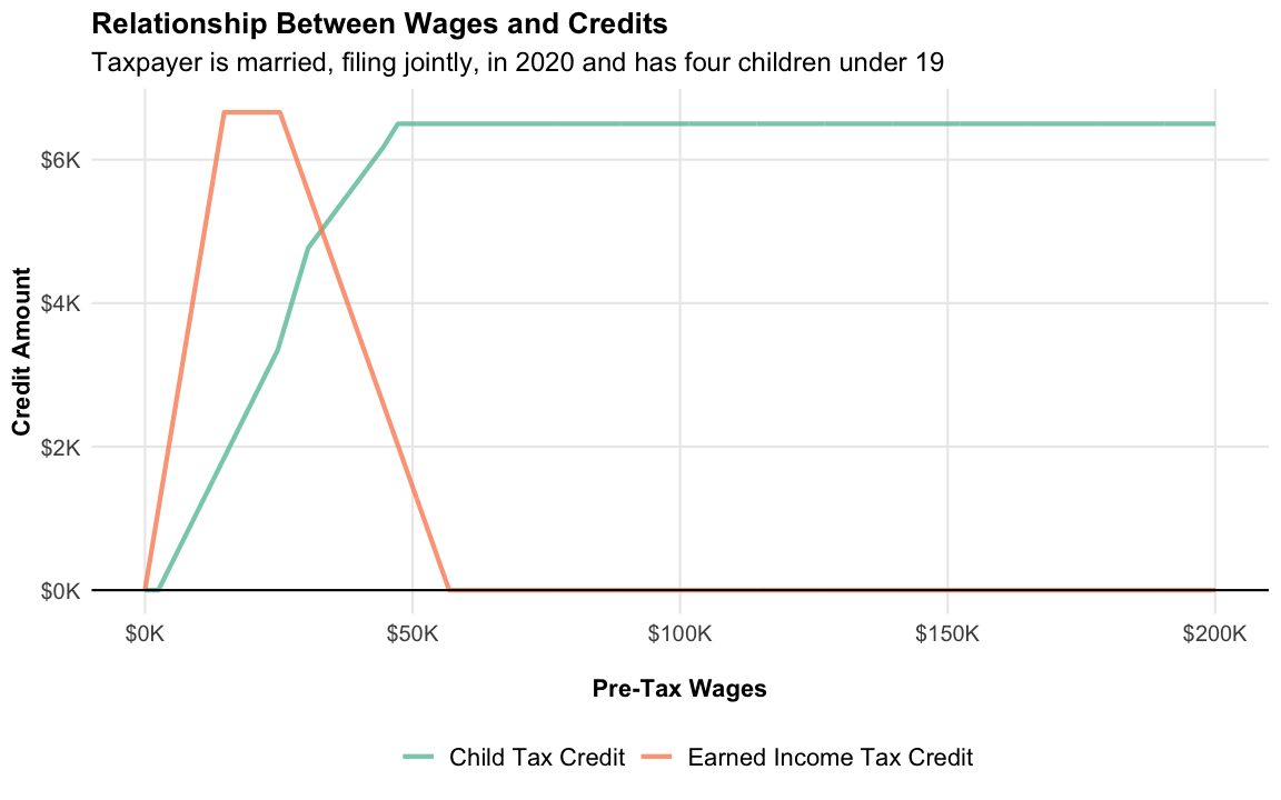
Credit and EITC. Let’s look at the amounts for both credits, while
varying household wages. The values reflect a household with four
children 18 or younger.
tax_items_mapping <- c(
  v25_eitc = 'Earned Income Tax Credit',
  child_tax_credit = 'Child Tax Credit'
)

family_income %>%
  filter(depx == 4) %>%
  mutate(child_tax_credit = v22_child_tax_credit_adjusted + v23_child_tax_credit_refundable) %>%
  select(pwages, fiitax, v25_eitc, child_tax_credit) %>%
  pivot_longer(cols = names(tax_items_mapping), names_to = 'tax_item', values_to = 'amount') %>%
  mutate(tax_item = recode(tax_item, !!!tax_items_mapping)) %>%
  taxes_line_plot(pwages, amount, tax_item) +
  labs(
    title = "Relationship Between Wages and Credits",
    subtitle = "Taxpayer is married, filing jointly, in 2020 and has four children under 19",
    x = "\nPre-Tax Wages",
    y = "Credit Amount",
    color = NULL
  )